 MathCS.org - Statistics
4.2 Measures of Central Tendency: Mean, Median, and Mode
While charts are frequently very useful to visually represent data, they are inconvenient for the simple reason that they are difficult to display and can not be remembered "by heart". It is frequently useful to reduce data to a couple of numbers that are easy to remember, easy to communicate, yet capture the essence of the data they represent. The mean, median, and mode are our first examples of such computed representations of data, and we will discuss how to compute each one and how to use Excel to simplify the calculation.
The Mean
The mean represents the average of all observations. It describes the "quintessential" number of your data by averaging all numbers collected. The formula for computing the mean is easy:
mean = (sum of all measurements) / (number of measurements)
In statistics, two separate letters are used for the mean:
- the Greek letter
 (mu)
is used to denote the mean of the entire population, or
population mean
(mu)
is used to denote the mean of the entire population, or
population mean - the symbol
 (read as "x bar") is used to denote the mean of a sample, or
sample mean
(read as "x bar") is used to denote the mean of a sample, or
sample mean
Another way to show how the mean is computed is:
where n stands for the number of measurements, x stands for the
individual measurements, and the Greek symbol sigma stands for "sum
of". That formula is valid for computing either the population mean
![]() or the
sample mean
or the
sample mean
![]() .
.
Of course, the idea - ultimately - is to use the sample mean
![]() as an
estimate for the population mean
as an
estimate for the population mean
![]() (which
is usually not known). For now, we will just show examples of
computing a mean, and later we will discuss in detail how exactly
the sample mean can be used to estimate the population mean.
(which
is usually not known). For now, we will just show examples of
computing a mean, and later we will discuss in detail how exactly
the sample mean can be used to estimate the population mean.
Example: A sample of 7 scores from people taking an achievement test were taken. The numbers are:
95, 86, 78, 90, 62, 73, 89
Then the mean of that sample is:
Excel actually provides a simple function for computing averages, namely the
=average(RANGE)
function. Using Excel, we can simply compute the above mean by entering the seven data observations into a new spreadsheet, then find a convenient spot to display the average number, and finally entering the appropriate =average(RANGE) function, where RANGE should be replaced by the appropriate range of cells. Try it out now - the answer should of course be 81.9
Note: In Excel the =average(RANGE) function ignores cells containing no numeric data, i.e. cells that contain no data or text, do not contribute anything to the computation of the mean. Cells that contain a zero do, however, do contribute to the average.
The mean applies to numerical variables, and in some situations to ordinal variables. It does not apply to nominal variables.
The Median (or Middle Number)
The median is that number from a population or sample chosen so that half of all numbers are larger and half of the numbers are smaller then that number. The computation is actually different for an even or odd number of observations.
IMPORTANT: Before you try to determine the median you must first sort your data in ascending order.
Example: Compute the median of the numbers 1, 2, 3, 4, and 5.
The numbers are already sorted, so that it is easy to see that the median is 3 (two numbers are less than 3 and two are bigger).
Example: Compute the median of the numbers 1, 2, 3, 4, 5, and 6.
The numbers are again sorted, but neither 3 nor 4 (nor any other of the numbers) can be the median. In fact, the median should be somewhere between 3 and 4. In that case (when there are an even number of numbers) the median is computed by taking the "middle between the two middle numbers". In our case the median, therefore, would be 3.5 since that is the middle between 3 and 4, computed as (3 + 4) / 2.
Note that indeed three numbers are less than 3.5, and three are bigger, as the definition of the median requires.
For larger data sets, the median can be selected as follows:
- Sort all observations in ascending order
- If n is odd, pick the number in the (n+1)/2 position of your data
- If n is even, pick the numbers at positions n/2 and n/2 + 1 and find the middle of those two numbers
Note that this does not mean that the median is (n+1)/2 (if n is odd) but rather that the median is that number which can be found at position (n+1)/n.
The median is usually easy to compute when the data is sorted and there are not too many numbers. For unsorted numbers, or for lots of numbers, the median becomes quite tedious, mainly because you have to sort the data first. But of course Excel has a built-in function
that will automatically compute the median of the numbers in a given range of cells.=median(RANGE)
Note: In Excel the =median(RANGE) function ignores cells containing no numeric data, i.e. cells that contain no data or text data, do not contribute anything to the computation of the median. Also, for an even number of numbers the median is automatically computed to be the middle between the two middle numbers.
The median applies to numerical variables, and in some situations to ordinal variables. It does not apply to nominal variables.
Discussion Topic: Discuss how to find the mean and the median of ordinal data, and why neither of these descriptive parameters makes any sense for nominal variables.
The Mode
The mode is that observation that occurs most often. It is usually not unique, and is therefore not that often used, but it has the advantage that it applies to numerical as well as categorical variables. As with the median, the mode is easy to find if the data is small and sorted:
Example: Scores from a test were: 1, 2, 2, 4, 7, 7, 7, 8, 9. What is the mode?
The mode is 7, because that number occurs more often than any other number.
Example: Scores from a test were: 1, 2, 2, 2, 3, 7, 7, 7, 8, 9. What is the mode?
This time the mode is 2 and 7, because both numbers occur three times, more than the other numbers. Sometimes variables that are distributed this way are called bimodal variables.
For data that consists of lots of numbers, and/or data that is not sorted, the mode, as the median, is cumbersome to compute by hand. Of course Excel provides an appropriate formula, in this case the
=mode(RANGE)
function. However, if the cell range consists several numbers with the same frequency (i.e. a bimodal variable as in the second example above) then the Excel =mode(RANGE) function returns only the first (smallest) number as the mode.
If all values occur exactly once, the Excel mode function returns N\A for "not applicable".
Mean, Median, and Mode: Pros and Cons
Since there are three measures of central tendency (mean, median, and mode) it is natural to ask which of them is most useful (and as usual the answer will be ... "it depends" -:)
The usefulness of the mode is in the fact that it applies to any variable. For example, if your experiment contains nominal variables then the mode is the only meaningful measure of central tendency (you could of course use frequency histograms to represent your data, as discussed in the previous chapter).
Mean and median usually apply in the same situations, so it is more difficult to determine which one is more useful. To understand the difference between median and mean, consider the following example:
Example: Suppose we want to know the average income of parents of students in this class. To simplify the calculations and to obtain the answer quickly, we randomly select 3 students to form a random sample. Let us consider two possible scenarios:
- Case 1: The three incomes may be, say, 25,000, 30,000, 35,000
- Case 2: The three incomes may be, say, 25,000, 30,000, 1,000,000
Compute mean and median in each case and discuss which one is more appropriate.
The actual computations are pretty simple.
- In case 1 the mean is 30,000 and the median is also 30,000.
- In case 2 the mean is 351,666, whereas the median is still 30,000
Clearly we were unlucky in case 2: one set of parents in this sample is very wealthy, but that is - probably - not representative for the students of the class. However, we selected a random sample, so scenario 1 is equally likely as scenario 2. Therefore it seems that the median is actually a better measure of central tendency than the mean, especially for small numbers of observations. In other words:
- the mean is influenced by extreme values, more so than the median
- the median is more stable and is the better measure of central tendency
However, for large sample sizes the mean and the median tend to be close to each other anyway, and the mean does have two other advantages:
- the mean is easier to compute than the median since it does not require sorted observations
- the mean has nice theoretical properties that make it more useful than the median
We will use both mean and median in the remainder of this course, while the mode will be less useful for us and will usually be ignored.
Exercise: Find the mean, mode, and median of the salary of Major League Baseball players. Why are the so different? Which one best represents the measure of central tendency? Did we compute the population mean (or median) or the sample mean (or median)?
major leagure baseball salaries
- mean = $1,916,817
- mode = not unique
- median = $565,000
- Mean and median are different because the data is not normal (symmetric). It is skewed to the right and therefore the mean will be larger than the median.
- As always for skewed data, the median is the "best" measure of central tendency.
Incidentally, the measures of central tendency computed above represent population measures, since they took all major league baseball players into account. Had I only used a subset of players to compute mean, mode, and median, the values would be sample measures.
Mean and Median for Ordinal Variables
As I mentioned, the mean and median work best for numerical values, but you can compute them, in a matter of speaking, for ordinal variables as well.
Example: Suppose you want to find out how students like a particular statistics lecture, so you ask them to fill out a survey, rating the lecture "great", "average", or "poor". The 14 students in the class rank the lecture as
"great", "great", "average", "poor", "great", "great", "average", "great", "great", "great", "average", "poor", "great", "average"
Compute the mean, the mode, and the median.
Obviously the mode is "great", since that is the most frequent response. For the other measures of central tendency I have to introduce numeric codes for the responses. I could define, for example:
"great" = 1, "average" = 2, and "poor" = 3
Then my data is equivalent to
1, 1, 2, 3, 1, 1, 2, 1, 1, 1, 2, 3, 1, 2
Now it is easy to see that the average is 22 / 14 = 1.57 and the median is 1.
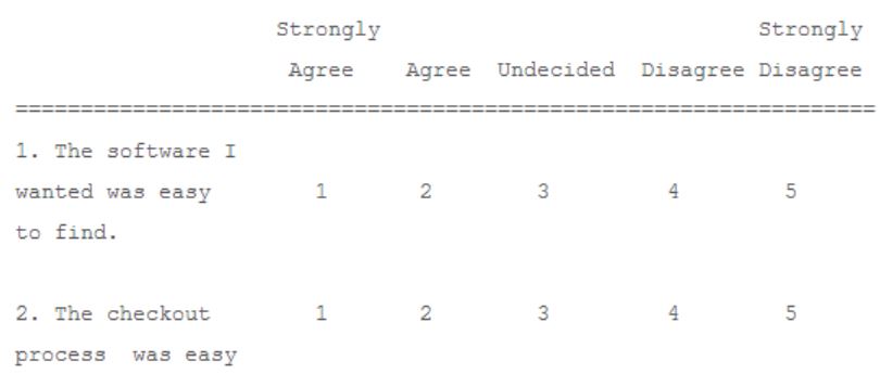
Of course the actual values for these central tendencies depend on the numeric code I am using for the orginal variables . I would need to justify or at least mention the codes I am using in a report so that the answers can be put in proper context. In a proper survey I would in fact list the code values together with the responses. One particular type of response that is frequently used in surveys is a Likert scale.
A Likert scale is a sequence of items (responses) that are usually displayed with a visual aid, such as a horizontal bar, representing a simple scale.
Mean, Mode, and Median for Frequency Distributions
We have seen how to compute mean, mode, and median for numeric data, and how to create frequency tables for categorical variables and histograms for numeric ones. As it turns out, it is possible to compute these measures of central tendency even if only the aggregate data in terms of a frequency table or histogram is available.
Example: Previously we looked at the heights of widgets produced in a certain factory:
3, 2, 5, 1, 4, 11, 3, 8, 23, 2, 6, 17, 5, 12, 35, 3, 8, 23, 6, 14, 41, 7, 16, 47, 8, 18, 53, 10, 22, 65, 9, 20, 59
We constructed a frequency table as follows from this data:
Category Count 13.8 and less 19 between 13.8 and 26.6 8 between 26.6 and 39.4 1 between 39.4 and 52.2 2 bigger than 52.2 3 Total 33 Based soley on this table, estimate the mean and compare it with the true mean of the full data set.
If all we knew was this table, we argue as follows:
- 19 data points are between 1 and 13.8, that is 19 data points are averaging (1+13.8)/2 = 7.4
- 8 data points are between 13.8 and 26.6, that is 8 data points are averaging (26.6+13.8)/2 = 20.2
- 1 data point is between 26.6 and 39.4, or 1 data point averages (26.6+39.4)/2 = 33.0
- 2 data points average (39.4+52.2)/2 = 45.8
- 3 data points above 52.2, or between 52.2 and 65.0, so that 3 data points average (52.2+65)/2 = 58.6
Thus, we could estimate the total sum as:
19*7.4 + 8*20.2 + 1*33 + 2*45.8 + 3*58.6 = 602.6and therefore the average would be approximately 602.6/33 = 18.26. The true average of the original data is 17.15. Thus, our estimate average is pretty close to the true average.
Of course if you had the original data, you would not need to do this estimation - you would of course use that data to compute the mean. But there are cases where you only have the aggregate data in table form, in which case you could use this technique to find at least an approximate value for the mean.
Example: A study of salaries of graduates from a University shows their income as follows:
Salary Range Count $7,200 - $18,860 130 $18,860 - $30,520 698 $30,520 - $42,180 254 $42,180 - $53,840 16 $53,840 - $65,500 2 Estimate the average incoming. Hint: you may use the following table (of course together with Excel) to get organized.
Salary Range range midpoint Count product $7,200 - $18,860 13030 130 1693900 $18,860 - $30,520 24690 698 17233620 $30,520 - $42,180 36350 254 9232900 $42,180 - $53,840 48010 16 768160 $53,840 - $65,500 59670 2 119340 Total 1100 29047920 To estimate the average, we compute the blue values in the above table. Then we divide the sum of the products by the sum of the counts to get as average 29047920/1100 = $26,407.20
There is no way to determine the actual average from this table, since you don't really know how the numbers fit into the various intervals. We would need access to the original raw data to find the true mean. It turns out, though, that the true average, using the original data is $26,064.21 which is indeed close to our estimate. In a similar way you can compute the mean of an ordinal variable. Try some problems.
That settles finding the mean, but how do we find the median or the mode? Well, that is actually much easier than the mean:
- compute the percentages for the frequency table: the category with the largest percentage is the mode
- add a column named "cumulative percent" to the frequency table by computing the sum of all percentages of all categories below the current one: the median is the first category where the cummulative percent is above 50%
Example: Find the median and the mode of the following salary table
Salary Range Count $7,200 - $18,860 130 $18,860 - $30,520 698 $30,520 - $42,180 254 $42,180 - $53,840 16 $53,840 - $65,500 2 We add two columns to the table: one containing the frequency as percent and the second containing the cummulative percent:
Salary Range Count Percent Cummulative % $7,200 - $18,860 130 130/1100 = 11.8% 11.8% $18,860 - $30,520 698 698/1100 = 63.5% 63.5+11.8 = 75.3% $30,520 - $42,180 254 254/1100 = 23.1% 75.3+23.1 = 98.4% $42,180 - $53,840 16 16/1100 = 1.4% 98.4+1.4=99.8% $53,840 - $65,500 2 2/1100 = 0.2% 99.8+0.2=100% Total 1100 100% We can now see that the mode is the 2nd category $18,860-$30,520, since it occurs most often at 63.5% and the median is also the 2nd category, since it is the first one where the cummulative percent is above 50%.
Note that finding the median depends on the fact that the categories are ordered, of course, which means that the variable is ordinal (or numeric in case of a histogram).