StatCrunch Manual
StatCrunch Overview
Version 0.9
Bert G. Wachsmuth
Contents
Summary
Statistics (mean, median, standard deviation, etc.)
How
to export/copy your results
Chi
Square test of independence
Finding
a regression line and correlation
Confidence
intervals about the mean
Introduction
StatCrunch is an online program for statistical analysis. It offers many advanced statistical features but is geared towards a student audience. While other programs such as SPSS are aimed at providing professional data analysis and reporting tools, StatCrunch’s strength is simplicity, ease of access, and ease of use. StatCrunch is entirely web based; even data sets and results are saved automatically to your online account and are available even if you use a different computer. However, you must be connected to the Internet to use StatCrunch.
How to start StatCrunch
Before you can use StatCrunch for the first time you must obtain a StatCrunch user ID and password. You can either redeem the license code that came with your text book or purchase a separate StatCrunch license using a credit card:
1. Start your web browser (either Internet Explorer, Firefox, or Safari)
2. Visit http://www.statcrunch.com/
3. Click Sign-in or Register on the top right of the screen
4. If you have an access code that came with your text book, click Redeem access code. Note that each
access code can be redeemed only once.
If your book did not include a valid
access code, you can purchase a new access code valid for 6 months.
5. Follow the online instructions to obtain your registration information. You will need to choose a user ID and a password. As user ID please use your email address. The password you choose is independent from any other of your passwords - make sure to remember it!
Assuming you received your StatCrunch user ID and password
(see above) you can access StatCrunch as follows:
1. Start your web browser (either Internet Explorer, Firefox, or Safari)
2. Visit http://www.statcrunch.com/
3. Enter your user ID: (as selected during registration, see above)
4. Enter your password: (as selected during registration, see above)
Click “sign in” - if all goes well you should see the StatCrunch main window:
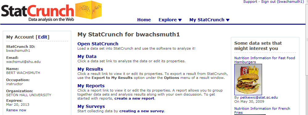 <
<
StatCrunch requires a web browser with Java enabled. If you have problems, contact the help desk at x2222.
Getting around in StatCrunch
Once logged in you’ll find three tabs to help you navigate – only one (My StatCrunch) will prove to be useful to us.

· The Home tab will return you to the login screen – it is not useful
· The Explore tab lets you explore publically shared data sets, results, etc – it is not useful
· The My StatCrunch tab will return you to the main screen
o
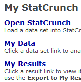 The My StatCrunch drop-down menu lets you access your data,
results, etc. directly.
Three additional links on the main menu – click on My StatCrunch to access - are important:
· Open StatCrunch: Load a data set to analyze or start with an empty set
· My Data: Shows you the data sets you saved previously
· My Results: Shows you any results you saved previously
How to enter Data
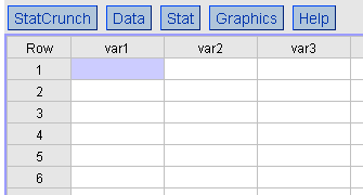 Click on My StatCrunch,
then Open my StatCrunch to start a
session with new data. You can enter data right into the spreadsheet by typing
it in, including editing the variable names, or you can import data from your
computer or from a web site.
To enter your own data
· Click on a variable name in the top row, use the backspace key to erase it, and type your own variable name
· Click on a cell in the spreadsheet and type or edit your data
· Press RETURN to advance to the cell below the current cell
· Select “Data | Save File” to save your data (frequently)
Import existing data
 You can import data in Excel
format or in “delimited” format,
either from a web site, from your computer, or from the clipboard. After you
upload your data set, it will be available in the My Data section. To import data from the web, first find a suitable
data file and copy its link (via right-click). Once you have the complete URL
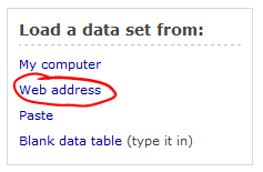
of your data set, click on Web address
in the “Load Dataset from” box on the left. Type the URL into the “WWW Address”
field that appears – or better, paste it via CTRL-V. Adjust the appropriate
options if necessary and click the “Load data” button.
Note: Data sets you upload are automatically saved and added to the My Data sections of your StatCrunch web account. Data that you typed in can be saved manually (select “Data | Save File”) and will also appear in My Data. To retrieve a data set you saved, visit My Data and click on the appropriate data set.
The GSS Sample Data
StatCrunch, like most computer programs, is best learned by exploring. You can use, for example, data from the General Social Survey (GSS) conducted in 2008. The General Social Survey (GSS) conducts basic scientific research on the structure and development of American society with a data-collection program designed to both monitor social change within the United States and to compare the United States to other nations. The GSS data sets contain a standard ‘core’ of demographic and attitudinal questions, plus topics of special interest, representing the population of American adults, 18 years of age or older. Many of the core questions have remain unchanged since 1972 to facilitate time trend studies as well as replication of earlier findings. The GSS takes the pulse of America, and is a unique and valuable resource. It is the only survey that has tracked the opinions of Americans over an extended period of time. The GSS is also a major teaching tool. There are over 14,000 research uses such as articles in academic journals, books, and Ph.D. dissertations based on the GSS and about 250,000 students annually who use it in their classes. More information about the GSS and its original data sets can be found through their web site.
At Seton Hall we have extracted 115 variables from the original GSS survey 2008 and recoded the data for use with a standard spreadsheet program such as Excel or the online stats package StatCrunch.
To load the main GSS dataset into StatCrunch:
1. Click on “My StatCrunch”
2. Select “Open StatCrunch”
3. Click “Web Address” on the left
4. Type http://mathcs.org/statistics/datasets/gss2008-short.xls into the web address field
5. Press ENTER or click the “Load” button at the bottom of the page
You now have a large, interesting data set to analyze. Note that the data set has been saved to the “My Data” section of StatCrunch. Next time you login to StatCrunch you can simply open the data set from there.
Additional data sets suitable for importing into StatCrunch can be found at http://www.mathcs.org/statistics/datasets or on the Blackboard site for your course.
Summary Statistics (mean, median, standard deviation, etc.)
Summary or descriptive statistics are numeric values describing a variable and its distribution. They include mean, median, variance, etc. They are appropriate for numeric variables. To obtain summary statistics:
- Load the GSS sample data set or open it from “My Data”
- Click on “Stat”
- Select “Summary Stats”
- Select “Columns”
- Select one or more variables from the list by clicking on them. Clicking on an unselected variable selects it, clicking on a selected one de-selects it. Note that you will see only the numeric variables in the list. Select, for example, AGE from the GSS 2008 data set
- The “Where” clause allows you to select subsets of the selected variables”, while the “Group by” clause allows you to group summaries into groups. Ignore these options and click “Next”
- Now you can select the descriptors you want. You can leave the defaults in place and click on “Calculate”.
- You will see a table, containing the descriptors for your selected variable(s). In case you selected AGE you’ll see:
Summary statistics:
|
Column |
n |
Mean |
Variance |
Std. Dev. |
Std. Err. |
Median |
Range |
Min |
Max |
Q1 |
Q3 |
|
AGE |
2013 |
47.708397 |
301.0516 |
17.35084 |
0.38672173 |
47 |
71 |
18 |
89 |
34 |
60 |
- You can copy this table to “My Results” for future use – see the next section – or, if you no longer need the results, simply close that window.
How to export/copy your results
Every time you complete an analysis you have the option of saving your result for future use in a report. If you do, you can name your result and add comments so that you can later find it easily. Saved results are stored in the My Result section and can be printed or copied to a Word document from there at any time. Saved results are stored permanently in your StatCrunch account until you explicitly delete them.
To see how to export your results, compute some statistics such as the summary statistics for the AGE variable of the GSS 2008 survey, as described previously.
- In the window showing the results of your computation, click “Options”

- Select “Export to My Results (Save/Copy/Print)”
- A new window will open, allowing you to give a title to your results – so give them an appropriate title
- Press “Export”
Your results have now been saved to “My Results”, even after you logout of StatCrunch. After you collected some results and exported them you can copy them to another program such as MS Word to embed them into a report or paper:
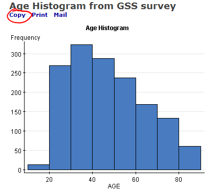
- Click on My StatCrunch to return to the main options
- Click on My Results to see a list of all your results
Results will be listed in the order they were created, newest one first. They will continue to be available any time you login to StatCrunch, until you explicitly delete them.
3. Click on the result you wish to transfer to MS Word
4. Click the “Copy” link near the title of your result to copy it to the clipboard (the first time you do this you may need to explicitly allow this operation –follow the instructions)
Now switch to the program into which you want this result to go, such as MS Word, and select Paste.
You might want to delete old results from your “My Results” area if you no longer need them.
Frequency Distributions
A frequency distribution shows how often items, numbers, or a range of numbers occur. It usually is given in form of a table, but could be represented graphically as well. They are appropriate for nominal or ordinal variables, or for numeric variables with a small number of distinct values. To obtain a frequency table:
- Load the GSS sample data set or open it from “My Data”
- Click on “Stat”
- Select “Tables”
- Select “Frequency”
- Select one or more variables from the list by clicking on them. Clicking on an unselected variable selects it, clicking on a selected one de-selects it. Select, for example, SEX from the GSS 2008 data set
- The “Where” clause allows you to select subsets of the selected variables”. Ignore this optional clauses and click “Next”.
- The next options can be ignored, click “Calculate”
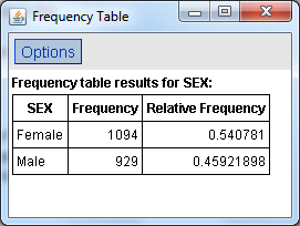
You will see that 1094 respondents were female and 929 were male. Out of a total of 1094 + 929 = 2023 that makes for a relative frequency of 0.54 or 54% for females and 0.46 or 46% for males. You could optionally copy your result to “My Results” for later use. Note that the GSS survey includes N = 2024 data sets so that one person chose not to answer the question about SEX. That person is considered “missing” and does not figure into the computation of the relative frequencies.
Graphs
It is often useful to obtain a graphical summary of the variables in your data. StatCrunch offers many choices, such as bar charts, pie charts, histogram, stem-and-leaf plots, box plots, and more. The type of chart to pick depends on the type of variable (numeric or categorical) and on what you are trying to accomplish. We will give two examples here:
Creating a box plot
- Load the GSS sample data set or open it from “My Data”
- Click on “Graphics”
- Select “Bar Plot”
- Select “with data”
- Select one or more variables from the list by clicking on them. Clicking on an unselected variable selects it, clicking on a selected one de-selects it. Select, for example, SEX from the GSS 2008 data set
- The “Where” clause allows you to select subsets of the selected variables”, while the “Group by” clause allows you to group summaries into groups. Ignore these optional clauses and click “Next”
- On the next dialog change ”Frequency” to “Relative Frequency” and select “Next”
- Now you can label the x or y axis and provide a title to your plot. Enter “Sex distribution in GSS 2008” as title, then click “Compute”
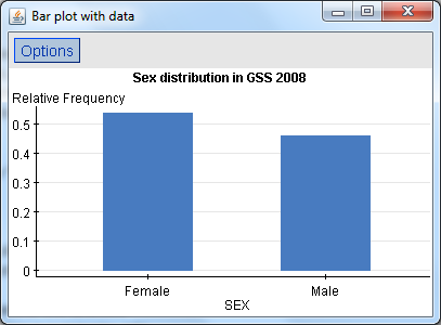
You will see a graphical representation of the frequency distribution for this variable.
Creating a Histogram
Histograms are suitable for numeric variables by placing their values into groups (also called “bins”). To create a histogram:
- Load the GSS sample data set or open it from “My Data”
- Click on “Graphics”
- Select “Histogram”
- Select one or more variables from the list by clicking on them. Clicking on an unselected variable selects it, clicking on a selected one de-selects it. Note that you will see only the numeric variables in the list. Select, for example, AGE from the GSS 2008 data set
- The “Where” clause allows you to select subsets of the selected variables”, while the “Group by” clause allows you to group summaries into groups. Ignore these optional clauses and click “Next”
- Change “Frequency” to “Relative Frequency”. You can optionally specify the bin width but the default usually works fine so click “Next”
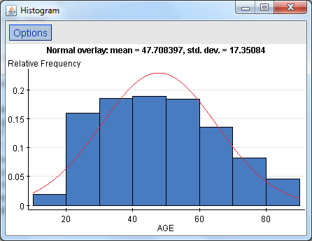
- Now you can overlay a standard distribution curve such as a normal curve to see if your variable can be approximated by that curve. Pick, in our case, “Normal” as your option and leave the rest alone. Click “Next”.
- You can again provide axis labels and titles, optionally, or click “Create Graph” to accept the defaults.
Contingency tables
A contingency table is used to explore a possible relationship between two variables. One variable is designated as row variable, the other as column variable, and the cells of the resulting table contain the number of values in that particular row and column. Contingency tables are most useful if both variables are categorical or better yet, ordinal (for two numeric variables one would use a regression analysis instead).
- Load the GSS sample data set or open it from “My Data”
- Click on “Stat”
- Select “Tables”
- Select “Contingency” and click on “with data”
- Next specify the row and column variables. Select, for example, SEX (one of the first few variables) as row variable and GENERAL HAPPINESS (one of the last few variables).
- Leave the “where” and “group by” entries alone and click “Next”
- Check “Row percent” and “Column percent” in the following dialog, then click “Calculate”
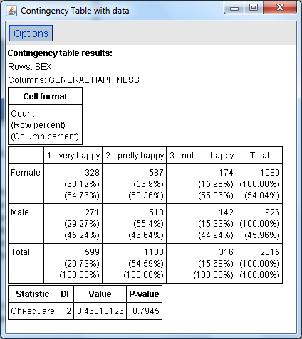
You will see, for example, that 30.1% of all females are very happy (row percent), while 44.94% of all “not too happy” people where male (column percent). Moreover, it seems like the overall happiness is not related to the sex of the respondents.
Note that a contingency table also computes the chi-square statistics for a test of independence. In this case, the p-value for the test is 0.7945 (which makes the test inconclusive).
Chi Square test of independence
To conduct a chi-square test for independence, compute a contingency tables as described previously.
Finding a regression line and correlation
A linear regression analysis checks if there a linear relation between two numeric variables.
- Load the GSS sample data set or open it from “My Data”
- Click on “Stat”
- Select “Regression”
- Select “Simple linear”
- Next specify the X and Y variables. Usually X is considered the independent variable, Y the dependent one. Note that only numeric variables are shown. Select, for example, FATHER HIGHEST YEAR SCHOOL as X variable and HIGHEST YEAR SCHOOL as Y to see if the number of years the father spent in school correlates linearly with the respondent’s years spent in school. Then click “Next”.
- You can now, optionally, enter a value for X to be used to predict Y, but in our case just click “Next”.
- Now you have a choice of graphics. Check “Plot the fitted
line” then press “Calculate”
You will see the numeric results, and if you press “Next” the plot of the least-square regression line.
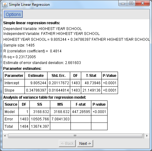
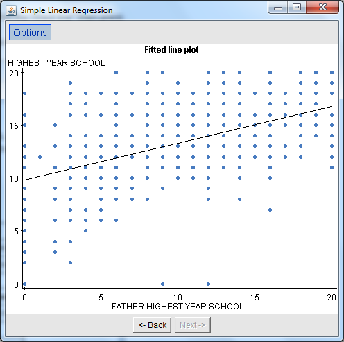
You can see, for example, that the equation of the least-square regression line would be:
Y = 0.348 * X + 9.805
but that the fit of the line to the data is not that great.
Confidence intervals about the mean
A 90%-confidence interval about the mean tells you an interval, i.e. lower and upper value, within which the true (unknown) population mean is located with 90% certainty. Other common confidence intervals are a 95% and a 99% confidence interval.
- Load the GSS sample data set or open it from “My Data”
- Click on “Stat”
- Select either “Z Statistcs” (for large data sets) or “T Statistics” (for small data sets). In our case the GSS data is large so pick “Z Statistics”.
- Select “One Sample”, then “with data”
- Next select the variable. Note that only numeric variables are shown. Select, for example, HOURS PER DAY WATCHING TV (near the bottom of the list).
- Leave the other options as they are and click “Next”.
- Check the “Confidence Interval” option and enter the interval you like, in our case 0.9 for a 90% confidence interval. Then click “Calculate”.
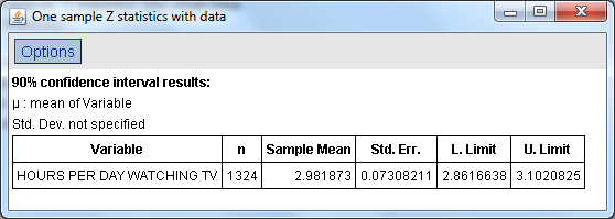
Our result means that the number of hours adults in the USA (the population for the GSS survey) watch TV is between 2.86 and 3.1 hours, with 90% certainty. The sample mean (of 2.98) is (always) in the middle of that interval. Note that n = 1324 indicates that 1324 (out of the GSS total of 2024) respondents answered this question.
 MathCS.org - Statistics