 MathCS.org - Statistics
back | next
6.3 Linear Regression
This time we again want to look at data from two variables that are possibly related, but we want to determine the exact nature of that relationship, if any, and develop some formulas that will allow us to make predictions. Let's use the same example that we have used before:
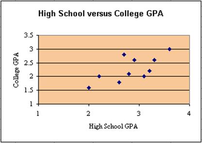
Example: A group of 11 students was selected at random and asked for their high school GPA and their freshmen GPA in college the subsequent year. The results were:
Student High School GPA Freshmen GPA 1 2.0 1.6 2 2.2 2.0 3 2.6 1.8 4 2.7 2.8 5 2.8 2.1 6 3.1 2.0 7 2.9 2.6 8 3.2 2.2 9 3.3 2.6 10 3.6 3.0
We would like to know whether there is a linear relationship between the high school GPA and the freshmen GPA, and we would like to be able to predict the freshmen GPA, if we know that the high school GPA of another student is, say, 3.4. In the previous section we came up with a scatter plot for this data:
Now we want to fit a straight line through these data points in such a way that the line "fits the data the best". We will specify in a second what we mean by "fits best", but for now let's look at three examples:
Line 1
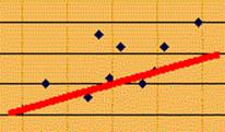
Line 2
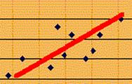
Line 3
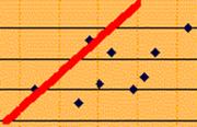
In each case we have drawn a line that somehow passes through at least some of the data points. It seems clear that:
- no straight line can pass through all data points exactly
- line 1 does not fit the data points very well because too many points are the the right, or below that line
- line 2 does not fit the data points very well because too many points are above the line
- line 3 does not fit the data points perfectly, but seems to have the best fit of these three lines
Mathematically speaking, the line that gives the "best fit" is that line where the sum of the squares of the differences to all data points has the smallest possible value. Therefore, the line that fits best in that sense is called least-square fit and the process of finding that line is called least-square linear regression.
The actual formulas involved are somewhat complicated, again, since they are based on the expressions Sxx, Syy, and Sxy we computed while working on the correlation coefficient.
Determining the Least Square Regression Line "manually"
Our goal is to determine the equation of the "least-square regression" line. In other words, we want to find the equation of a line (which happens to be called "least-square regression line"). We know from high school that a line has the equation:
y = m x + b
where m is the slope of the line, and b is the interception of the line with the y-axis. We also recall from high school that lines that go up have a positive slope (as the lines 1, 2, and 3 above), while lines with negative slopes go down.
Example: Suppose we have four equations of lines as follows:
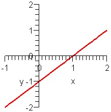
- y = x - 1
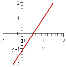
- y = 2x - 1
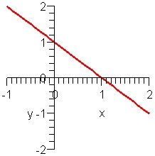
- y = -x + 1
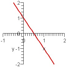
- y = -2x + 1
Moreover, let's say we have four graphs of lines, as follows:
Graph A
Graph B
Graph C
Graph D
Which graph matches what equation?
Solution: According to the equations of the lines, we have the following information:
- y = x - 1 is a line with slope 1 (going up) and y-intercept -1
- y = 2x - 1 is a line with slope 2 (going up) and y-intercept -1
- y = -x + 1 is a line with slope -1 (going down) and y-intercept 1
- y = -2x + 1 is a line with slope -2 (going down) and y-intercept 1
Graphs A and D show lines going up, so both have positive slope. Both also intersect the y-axis at -1, so both have y-intercept -1. But the line in graph D is steeper, so it should have a bigger slope. Thus:
- equation 1matches graph A
- equation 2 matches graph D
Similarly, both graph B and C have negative slopes and y-intercept +1, but line C goes down faster and thus has a more negative slope. Therefore:
- equation 3 matches graph B
- equation 4 matches graph C
So to determine the least-square regression line we must find the equation of a line with its the slope m and y-intercept b. As it happens, the slope is related to our quantities Sxx, Syy, and Sxy we computed earlier, while the y-intercept is related to the averages (means) of x and y. The formulas are as follows:
- Slope m = Sxy / Sxx
- y-Intercept b = (mean of y) - (mean of x) * m
where
-
-
-
- mean of x = (sum of x) / n
- mean of y = (sum of y) / n
In this class we are will not try to determine how these formulas come about. That would be done in more advanced math courses. We will be content using these questions, as in our next example.
Example: Consider the above data of high school versus college GPA and compute the equation of least square regression line. Also compute the correlation coefficient.
Solution: just as we did for the correlation coefficient in the first section, we make a table of x, y, x2, y2, and xy values:
Student x y x2 y2 xy 1 2.0 1.6 4.00 2.56 3.20 2 2.2 2.0 4.84 4.00 4.40 3 2.6 1.8 6.76 3.24 4.68 4 2.7 2.8 7.29 7.84 7.56 5 2.8 2.1 7.84 4.41 5.88 6 3.1 2.0 9.61 4.00 6.20 7 2.9 2.6 8.41 6.76 7.54 8 3.2 2.2 10.24 4.84 7.04 9 3.3 2.6 10.89 6.76 8.58 10 3.6 3.0 12.96 9.00 10.80 Totals 28.4 22.7 82.84 53.41 65.88
Thus, we can compute:
- Sxx = 82.84 - 28.42/10 = 2.184
- Syy = 53.41 - 22.72/10 = 1.881
- Sxy = 65.88 - 28.4*22.7/10 = 1.412
We also can quickly compute (since we already know the sums of x and of y):
- mean of x = 28.4/10 = 2.84
- mean of y = 22.7/10 = 2.27
But now the difficult work is over and we can compute the slope and y-intercept, as well as correlation coefficient, easily:
- slope m = Sxy / Sxx = 1.412 / 2.184 = 0.645
- y-intercept b = (mean of y) - (mean of x) * m = 2.27 - 2.84 * 0.645 = 0.4382
- correlation coefficient r = 1.412 / sqrt(2.184 * 1.881) = 0.6966
Thus, the equation of our least-square regression line, relating high school GPA (x) and college GPA (y) is:
- y = 0.645 * x + 0.4382
and the correlation coefficient of 0.6966 indicates that the relation is not very strong.
We can now use our computed equation to make predictions.
Example: Using the above data for high-school and college GPA's, predict the college GPA for a student with a high school GPA of 3.7.
Solution: First note that x = 3.7 is not one of the original high school GPA scores. But we know the general relationship between x and y (the equation of the least-square regression line) which we use for our prediction:
so that if x = 3.7 we have for y:
Thus, our prediction is that a high school GPA of 3.7 will result in a college GPA of 2.83, approximately. Moreover, because of our correlation coefficient we are relatively confident (but not super-confident) that our prediction is accurate.
This was a lot of work but before we use Excel for the heavy-duty computations, let's do one more example manually.
Example: Suppose some (made-up) data for two variables x and y is as shown in the table. Use that data to predict the y value for x = 5 and state how confident you are in your prediction:
x y 1 3 2 5 3 6
Solution: We create, as usual, a table of x, y, x2, ect. data, compute the Sxx, etc, and finish up with the equation of the line. Here are the results:
x y x2 y2 xy 1 3 1 9 3 2 5 4 25 10 3 6 9 36 18 Totals 6 14 14 70 31
- Sxx = 14 - 62/3 = 2
- Syy = 70 - 142/3 = 4.667
- Sxy = 31 - 6*14/3 = 3
We also can quickly compute
- mean of x = 6/3 = 2
- mean of y = 14/3 = 4.667 (it is a coincidence that this value matches the above for Syy.
But now the difficult work is over and we can compute the slope and y-intercept, as well as correlation coefficient, as follows:
- slope m = Sxy / Sxx = 3/2 = 1.5
- y-intercept b = (mean of y) - (mean of x) * m = 4.667 - 2*1.5 = 1.667
- correlation coefficient r = 3 / sqrt(2*4.667) = 0.982
Thus, the equation of our least-square regression line, relating x and y is:
- y = 1.5 x + 1.667
Thus, if x = 5 we compute our prediction to be y = 1.5 * 5 + 1.667 = 9.167 and since the correlation coefficient is 0.982 we think that the relation is very strong. Thus, we are pretty sure about our prediction.
Please note that we are basing our prediction or forecast on only 3 data points. Such a small sample is generally not adequate for good predictions. However, the three points are linearily related, so for better or worse we believe our prediction is good. A more careful analysis of the goodness of our prediction would involve probabilities and is beyond our scope at this time.
Determining the Least Square Regression Line "automatically"
After all this work it should be relating to focus on using Excel to deliver the least-square regression line for us.
- Start Excel as usual and enter the data from the above GPA example
- From the "Tools" menu, select the "Data Analysis ...." menu item and choose "Regression"
- In the "Regression" dialog window use the selector tools and select the X and Y range (be careful, the first range to choose is the Y range, not X). If you include the labels in the ranges, make sure to check the "Labels" box.
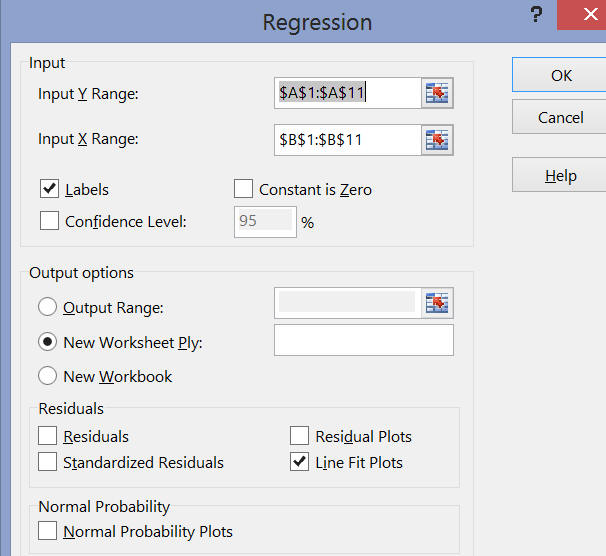
To get a scatter plot including the least-square regression line, make sure to check "Line Fit Plots" in the "Residuals" category. To connect the dots with the least-square regression line, double-click on a pink dot and check "Solid line" on the options on the right side after you generate the regression output.
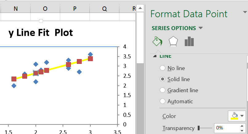
You can, as before, change the x and y axis scale, pick a background color, choose a title, set the line color, modify or remove the markers, etc. Experiment!
The Regression Analsysis actually produces a lot of output, much of it with mysterious sounding names. Here is the interpretation of the most important pieces of the output:
|
|
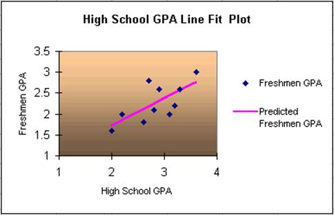
The Chart: includes the scatter plot as before (blue diamond-shaped dots), but also the "predicted" scores (pink rectangluar-shaped dots). If you connect these pink dots you obtain the least-square regression line. |
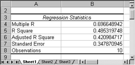
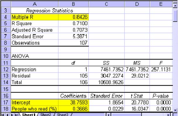
- The Regression Statistics: This statistics is also computed by the regression analysis and looks similar to the following:
The most important number here is "Multiple R" which has the value of 0.6966 in this case. In fact, that number is almost the same as the "correlation coefficient" introduced earlier. In fact, this "multiple R" is the absolute value of our previous correlation coefficient. Thus, multiple R is always between 0 and 1, and closer to 1 indicates stronger relation. Hence, in this case being resonably close to 1, implies that we can conclude that the two variables are indeed somewhat related. In other words, if the value or "Multiple R" in the "Regression Statistics" is close to 1, then the least-square regression line indeed fits the data points pretty well, and there is a linear (positive or negative) relation between the two variables. It does not indicate which way the relation goes, as the correlation coefficient does.
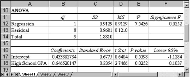
- The "Anova" Section: The next section produced by our regression analysis is the Anova (Analysis of Variance) section:
The two most important numbers in this section are the "Coefficients" for the "Intercept" and the "High School GPA". In this case "Intercept" is 0.4339 and "High School GPA" is 0.6465 (rounded). These two numbers are the slope and intercept of the least-square regression line. In other words, the actual equation of the least-square regression line is:
That equation of the line, in fact, can be used for predictions. For example, if we want to know the College GPA (Y) for a student with a high school GPA (X) of 3.4 - or, mathematically speaking, if we want to know the y value when x = 3.4 - we simply substitute x = 3.4 in the above equation and we find the corresponding y value to be
.
Note that from this section we see that the slope is positive, which means that the correlation coefficient is also positive. Thus, in this case the correlation coefficient and the multiple R are identical (if the slope had come out negative, the correlation coefficient would be -(multiple R), i.e. it would have been -0.6966).
|
|
The "Residual Output" Section: is not important for us in this lecture so we will ignore it. |
Now we can also answer the original question: based on our data and a least-square regression analysis of that data, we can predict that a student with a high school GPA of 3.4 will have a college GPA of approximately 2.632. Since the correlation coefficient is 0.69 we are reasonably confident that our prediction is accurate.
Summary of Regression Analysis:
To summarize a typical least-square regression analysis:
- Enter the data in columns in Excel or load an existing data set
- Choose "Regression" from the "Data Analysis ..." menu item in the "Tools" menu
- Select X (independent variable) and Y (dependent variable) ranges and any other options and click on "OK"
- Look at the "Multiple R" value in the "Regression
Statistics":
-
if that value is close to -1 or 1, there is a strong linear relationship between X and Y and the least-square regression line will fit the data well
-
if that value is close to 0, the least-square regression line (which is the best line possible) does not fit the data very well
-
-
Write down the equation of the least-square regression line in the form y = mx + b, where m is the slope (from the "Coefficient" column in the last row) and b is the y-intercept (from the the "Coefficient" column in the second-last row labeled "Intercept")
-
Use that equation of the least-square regression line to make predictions by substituting the desired x into the equation and computing the corresponding y value. The closer the "Multiple R" value is to 1, the more trustworthy the prediction is. You should always mention the "Multiple R" value when making a prediction. If you want to be sophisticated you should also indicate the value of the correlation coefficient if the slope is negative.
Here is another example, this time with real - and interesting - data:
Example: In the attached Excel spreadsheet you will find data about the literacy rate (percentage of people who read) and average life expectancy of about 100 countries in the world, based on 1995 data. Load that data into Excel and perform a least-square regression analysis to see if there is a linear relationship between the literacy rate and the average life expectancy. If you find that there is a relation, determine what would happen to the life expectancy of people in Afghanistan if the literacy rate could be raised to, say, 60% (from its current value of 29%).
The technicalities of the least-square regression analysis should be clear, so we will simply state and interpret the results: The least-square regression line fits the data quite well, as is clear from the scatter plot:
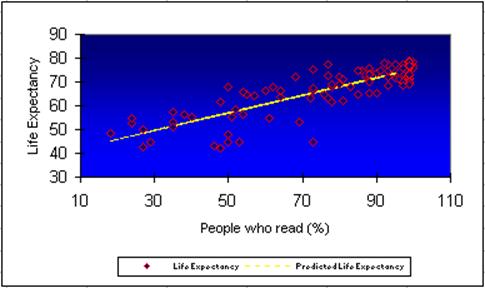
as well as from the value of the correlation coefficient 0.84 which can be found in the "Multiple R" section of the regression analysis output.
The coefficients of the least-square regression line are 38.7593 (intercept) and 0.3666 (slope) so that the line has the equation:
That means that if a country such as Afghanistan had a literacy rate of 60%, we would predict an average life expectancy of approximately y = 0.3666 * 60 + 38.7593 = 60.7553, or approximately 60 years (as opposed to its current life expectancy of 45 years. Since the correlation coefficient is 0.84 we are in fact quite sure that this prediction is accurate.
Note: This does not mean that reading books causes people to live longer. After all, at the beginning of analyzing two variables we mentioned that correlation does not necessarily imply causation. But what it does mean is that if a country can raise its literacy rate, probably through a wide variety of programs and policy decisions, then a beneficial side effect seems to be that the average life expectancy goes up proportionally as well. It also means that if a country - perhaps for political reasons - does not make its life expectancy rate public, but its literacy rate is known, we can give a pretty good estimate of that life expectancy based exclusively on the literacy rate of the country.